When Does Self-Hosted Inference Beat a Managed API? A 12-Month Operating Model

Self-hosted inference can have a lower modeled cost than a managed API while remaining an unready operating choice. The comparison needs a workload, a capacity assumption and an owner for the work that the API provider previously performed. A token price comparison supplies only part of that decision.

Use a twelve-month ledger for one defined workload. Keep the model's acceptance requirements constant, expose the step at which another serving pool is needed and leave unpriced operational work visible. Only then ask whether the modeled saving is large enough to justify gathering the missing evidence.

This article develops fictional scenario I-64. Every demand, capacity, staffing and dollar figure below is an illustrative assumption, not a supplier quote, hardware benchmark or client result. The arithmetic was calculated locally. No GPU workload, managed inference request or production recovery exercise was run.

Define the same useful workload on both sides

Start with the task that the application needs to complete. Record the model or candidate models, input distribution, output limits and acceptance criteria. A cheaper response that fails the application's review rules is a different outcome. Before comparing operating costs, establish what evidence would make the alternatives acceptable substitutes.

For I-64, one request-equivalent represents a hypothetical task with 1,000 input tokens and 250 output tokens. The ledger assumes that both alternatives complete the same task mix to the same required standard. That equivalence has not been tested. It is a prerequisite to investigate, rather than a conclusion produced by the spreadsheet.

Keep attempted requests separate from accepted task completions. Retries, evaluator calls and fallbacks can increase billed work without increasing the number of completed tasks. The simplified I-64 arithmetic initially assumes one attempt per task. An actual workbook should replace that assumption with observed counts and explain which categories enter each cost meter.

Token counts also need a common interpretation. A change of model or tokenizer can change the input count, output length and quality distribution. Do not carry a request-level unit cost from one candidate into another without checking the associated workload. A convenient average can hide the long requests that determine memory pressure and queue behavior.

Write down the arrival pattern as well as monthly volume. A workload of overnight batch jobs has different timing constraints from interactive requests arriving in a short peak. The ledger below uses monthly capacity as a simplifying assumption. It cannot demonstrate that a serving pool handles a specific burst or meets an interactive latency objective.

Name the operating boundary

In this comparison, self-hosting means that the application team owns the model-serving runtime and its operating responsibilities. The underlying compute may still be rented from a cloud provider. It does not require buying physical hardware. If hardware purchase is actually proposed, add its acquisition, maintenance and residual-value assumptions rather than treating the pool charge as a complete substitute.

Managed API means an externally operated model service with a workload-linked rate in this fictional ledger. A dedicated managed endpoint with reserved capacity may have a different billing shape. Do not apply the I-64 API column unchanged to that offer. First identify the relevant fixed commitments and variable meters, then calculate its own monthly subtotal.

A shared model name is not enough to settle the boundary. Ask who controls the runtime version, who investigates serving failures and who can change capacity. These answers determine which tasks remain with the buyer. They also identify the evidence needed before treating the offered service as a substitute for the proposed self-hosted path.

Keep the comparison narrow while collecting those answers. The application can retain its evaluation and business rules under either serving choice. This ledger compares the operating boundary of inference for the stated task; it does not decide ownership of the entire AI product.

Make every input's status visible

The first worksheet should contain the value, unit, source and confidence status of each assumption. Use observed values where evidence exists. Mark estimates as estimates and unknowns as unknowns. A cell containing zero is a numeric claim; it is not an appropriate substitute for a cost nobody has priced.

I-64 uses the following fictional inputs. Dollar amounts are illustrative USD and do not represent current market rates. The managed request-equivalent rate is a combined assumption for the stated input and output mix. It should be replaced by the actual applicable billing meters in a real comparison.

Input	Fictional I-64 value	Boundary
Managed cost per million request-equivalents	$2,000	Combined task-mix assumption
Self-hosted variable cost per million	$200	Assumed incremental operating meter
Serving pool cost per month	$3,000	Reserved capacity, billed even when idle
Capacity per pool per month	6 million request-equivalents	Unmeasured usable-capacity assumption
Other priced operations per month	$1,500	Limited placeholder, not complete staffing coverage
One-time setup	$9,000	Included once in month one
Minimum active pools	1	Does not establish high availability
Horizon	12 months	No residual asset value assumed

The operations placeholder needs particular care. It does not claim that $1,500 buys an on-call team, license review, security maintenance and every evaluation run. Those jobs remain in a separate unpriced register until an owner estimates them. Treat the result as a priced subtotal while that register is open.

For capacity, record what the number means before entering it. In I-64, six million is an assumed volume that one pool could serve within the still-unverified quality and timing conditions. It is not GPU utilization, a vendor throughput promise or a measured number of accepted outputs. The distinction prevents arithmetic from becoming accidental benchmark evidence.

Calculate the month, including idle capacity

For each month, divide request-equivalent demand by assumed pool capacity and round upward. Keep at least one pool. Multiply that pool count by its monthly price, then add the operations placeholder and variable cost. Add setup once. The managed subtotal is monthly demand multiplied by the assumed managed unit rate.

This model assumes that an additional pool is available when needed and can be billed for the relevant month. Procurement delay, minimum reservation terms and deployment time are not modeled. If those conditions apply, add them explicitly. A formula that can increase capacity instantly is not evidence that the team can obtain it instantly.

The demand path starts at 0.8 million request-equivalents and reaches 6.4 million in month twelve. The last month crosses the fictional six-million boundary and therefore requires two pools. Earlier idle capacity remains paid. The table reports priced subtotals before any unresolved operational additions.

Month	Demand, millions	Pools	Managed subtotal	Self-hosted subtotal
1	0.8	1	$1,600	$13,660
2	1.0	1	$2,000	$4,700
3	1.3	1	$2,600	$4,760
4	1.5	1	$3,000	$4,800
5	2.0	1	$4,000	$4,900
6	2.4	1	$4,800	$4,980
7	3.2	1	$6,400	$5,140
8	3.8	1	$7,600	$5,260
9	4.4	1	$8,800	$5,380
10	5.0	1	$10,000	$5,500
11	5.6	1	$11,200	$5,620
12	6.4	2	$12,800	$8,780
Total	37.4	13 pool-months	$74,800	$73,480

The self-hosted priced subtotal is $1,320 lower over the fictional year. That is an arithmetic difference, not a measured saving or a complete cost result. Setup makes the first month expensive; idle capacity dominates several early months; the additional pool changes the final month. An annual average alone would conceal that path.

Keep cash timing visible if it affects the decision. A team may be unable to accept a larger early commitment even when the eventual subtotal is lower. I-64 makes no financing or accounting recommendation. It simply keeps the setup payment and monthly capacity commitments attached to the months in which the model incurs them.

Find break-even within a capacity band

Within a fixed pool schedule, the difference between the two variable rates is $1,800 per million request-equivalents. With one pool for all twelve months, the modeled fixed subtotal is $63,000: setup plus twelve months of pool and operations costs. Dividing that fixed subtotal by the rate difference gives 35 million request-equivalents for the year.

That threshold is conditional on the one-pool schedule remaining feasible. It does not authorize unlimited demand through the same pool. If a monthly peak requires another pool, recompute the fixed subtotal. I-64 incurs thirteen pool-months, taking the fixed subtotal to $66,000 and the corresponding annual threshold to about 36.67 million.

The timing of demand therefore matters even if two workloads have the same annual total. One may fit its demand inside the existing pool each month; another may require temporary additional capacity. If the billing arrangement cannot release that capacity promptly, the fixed commitment can persist beyond the peak. Model the actual terms rather than assuming frictionless scaling.

This is why a single utilization percentage cannot serve as a universal purchasing rule. The decision depends on useful capacity, billing duration, setup and the cost difference per comparable task. A rule such as self-hosting wins above a particular GPU utilization level discards those inputs before the calculation begins.

Keep the threshold's units visible beside the answer. Here it is annual request-equivalents under a named pool schedule. In a token-based workbook, input and output meters may remain separate. In another system, the useful denominator may be reviewed documents or completed jobs. Do not exchange those units merely to produce a cleaner chart.

Change the capacity assumption before trusting the result

A capacity sensitivity table asks how much the conclusion depends on a number that has not been measured. Hold the fictional pool price and workload path constant, then vary usable capacity. This represents uncertainty about the same proposed serving arrangement, not an assertion that different hardware offers the same price.

Assumed capacity per pool-month	Required pool-months	Self-hosted priced subtotal	Difference from managed
3 million request-equivalents	19	$91,480	$16,680 higher
6 million request-equivalents	13	$73,480	$1,320 lower
9 million request-equivalents	12	$70,480	$4,320 lower

Under the six-million assumption, aggregate demand uses about 47.95 percent of the assumed paid capacity across thirteen pool-months. That is a worksheet ratio: demand divided by provisioned request-equivalent capacity. It is not measured GPU busy time, memory occupancy or evidence that latency remains acceptable at a particular load.

The nine-million assumption produces a lower subtotal despite a lower ratio of demand to provisioned capacity. The three-million assumption produces a higher subtotal despite greater use of its smaller assumed pools. This is a useful warning against comparing utilization ratios without their capacity definitions and cost terms.

Run a separate demand sensitivity after the capacity review. Slower growth leaves more reserved capacity idle. Faster growth may cross another billing step. Do not combine an optimistic demand forecast with an optimistic capacity estimate and call the resulting number a base case. Retain a named conservative scenario and explain which evidence would replace it.

Check quality and queueing before accepting capacity

Capacity should be investigated with the model, runtime settings and task distribution that the application intends to use. Define an acceptance dataset and timing objective before measuring. Record rejected responses and failures alongside successful requests. A throughput count without those boundaries cannot establish the useful capacity that the cost ledger assumes.

The vLLM per-request metrics documentation defines queue time as:

Time the request spent waiting in the scheduler queue before processing began.

That definition makes scheduler waiting a separate observation. It helps explain why a resource can remain busy while a user waits too long. The vLLM project also documents request latency and token-related measurements. Read each metric's scope before comparing it with application-level timing, especially where a measurement starts after scheduling.

For an interactive workload, measure the path the user experiences as well as server-side processing. Distinguish waiting, first useful output and completion. For a batch workload, specify the completion window and treatment of late jobs. These choices affect which measured capacity can legitimately enter the workbook.

Also preserve the tested configuration. Changing context length, output limits, batching, model version or quantization can alter both performance and task acceptance. An old benchmark number is not automatically portable to a new configuration. Record the change and reopen the relevant quality and capacity evidence before updating the cost claim.

I-64 leaves these gates unverified. Its table tells the team which assumptions are worth testing, not which model to deploy. A lower priced subtotal should lead to an evidence request before it leads to a production commitment.

Keep an unpriced-operations register beside the subtotal

Self-hosting moves responsibilities rather than making them disappear. The team needs someone to maintain the serving runtime, review model changes and handle degraded service. A managed API still leaves application integration, evaluation and provider coordination with the buyer. Put the remaining work on both sides into a register.

Open work	Evidence to request	Current I-64 state
Runtime and model updates	Owner, review process and estimated effort	Unpriced
Incident coverage	Coverage window, escalation and staffing estimate	Unpriced
Quality regression checks	Dataset, reviewer and rerun budget	Unpriced
Security and license review	Review scope and accountable owner	Unpriced
Fallback operation	Trigger, usable capacity and priced work	Unpriced
Provider or model migration	Expected handover and transition scope	Unpriced

Do not add these rows to zero and present the sum as total cost of ownership. The known subtotal and unresolved register are different outputs. A decision record should show both. Where the current comparison excludes taxes, storage, network transfer or a support arrangement, describe that exclusion explicitly rather than hiding it in a miscellaneous line.

The small I-64 difference shows why this matters. An additional fictional $200 per month of self-hosted work would add $2,400 over the year. The adjusted self-hosted subtotal would become $75,880, above the unchanged managed subtotal. That sensitivity is a calculation, not a claim about the actual price of any operational task.

Ask whether shared staff costs are incremental, allocated or already committed. Each treatment can answer a legitimate question, but mixing them makes the comparison misleading. If the decision is whether to add a service, incremental staffing matters. If the purpose is product cost allocation, a broader allocation may be appropriate. Name the question the ledger answers.

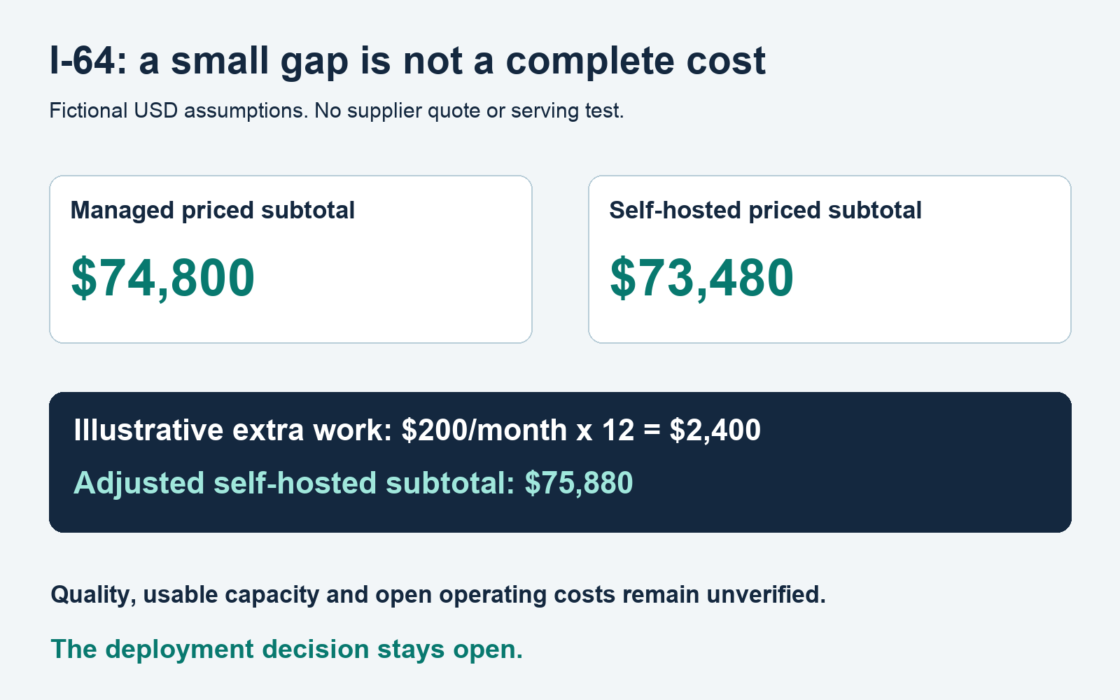
Fictional I-64 arithmetic. Illustrative USD inputs; no supplier quote or serving test.

Price the fallback that the design actually requires

A fallback path can consume API budget, spare self-hosted capacity or operator time. Record its trigger and the work it performs. If it repeats a request after an unknown result, the application may also need a safe treatment of duplicate downstream actions. Serving a model response and executing an external tool are separate boundaries.

Do not assume that one minimum pool provides high availability. A failure may remove that pool's entire usable capacity. If the design requires redundancy, include the additional capacity commitment and the evidence needed to exercise recovery. I-64's one-pool minimum is a simplifying assumption, not an availability architecture.

For a managed API, document relevant rate limits, service dependencies and the proposed alternative when the provider is unavailable. A second provider may produce different outputs or use different controls. Its existence alone does not establish task equivalence. Include the evaluation and integration work needed before it can serve as a credible fallback.

Keep fallback volume visible in the meters. A percentage of requests diverted to another service can change both variable cost and the peak load on the retained system. Model that branch separately before combining subtotals. Otherwise, the comparison may charge for the primary path while relying on an unpriced secondary path for reliability.

Keep the workbook reproducible

Save the inputs separately from the monthly formulas. Give every scenario a name and retain the assumption version with its output. A reviewer should be able to change pool capacity without editing the demand series or the managed rate. This makes the sensitivity a controlled change rather than a fresh collection of convenient inputs.

Check unit conversions at the boundary of each meter. I-64 stores demand in millions of request-equivalents, so its rates are also expressed per million. Multiplying those values produces dollars directly. If another worksheet stores individual requests, convert once and label the conversion. Repeating a million-unit conversion in several formulas makes a silent scale error harder to locate.

For each month, calculate the integer pool count before calculating its charge. Do not round the annual average and multiply it by twelve. That alternative would erase the month-twelve step in I-64. Preserve the one-time setup line separately so it cannot recur accidentally when the monthly table is copied into a new period.

Add simple reconciliation checks: monthly demand should sum to annual demand, pool counts should sum to billed pool-months and monthly subtotals should sum to the annual subtotal. These checks validate the workbook arithmetic. They cannot establish that its capacity, costs or acceptance assumptions describe an actual deployment.

Normalize cost only after acceptance is defined

When testing becomes available, add the count of accepted task completions to each path. Define who accepts a result and which failed or abandoned attempts remain billable. A system can generate many outputs while producing fewer usable task outcomes. A per-token comparison cannot resolve that distinction by itself.

Keep application review cost visible where it differs. If one candidate requires more human correction, the serving subtotal alone may understate the work needed to complete the task. Estimate that work through a documented review process rather than assigning an arbitrary penalty to the model you prefer less.

Recalculate when the acceptance rules change. A stricter output requirement may alter the usable capacity or the number of retries. Preserve the old calculation as a result for its original task definition, then create a new scenario. This prevents an apparently stable unit cost from hiding a moving definition of success.

Publish a decision record that can be reopened

A useful conclusion contains the workload version, horizon, priced subtotal, open costs and evidence gates. For I-64, the record would say that self-hosting has a $1,320 lower fictional priced subtotal under the six-million capacity assumption, while quality, usable capacity and several operating costs remain unverified. The deployment choice stays open.

Assign an owner to each unresolved input and specify what would resolve it. A price quote, measured scenario, staffing estimate and license review are different artifacts. They should not all collapse into one label saying more research is needed. The next action should be specific enough for the responsible person to accept.

Reopen the record when the workload or operating terms change. Examples include longer outputs, a different model, a new latency objective or a minimum capacity commitment. Preserve the old assumptions and result as history. A cost comparison cannot remain current if its defining task changes underneath it.

Commission the evidence before committing to the operating model

Pharos Production AI development services is a relevant starting point for discussing an AI application's architecture and implementation scope. Ask for a workload-bound evaluation and operating brief with explicit deliverables. A service description does not establish a measured serving capacity, a supplier price or a saving for your application.

Apply the same evidence requirements to a Pharos Production inference proposal as to any other proposed implementation. Require the task acceptance rules, capacity measurements and receiving-team responsibilities to be stated. Keep any discovery or implementation estimate separate from the fictional numbers in I-64.

If the unresolved decision is broader than serving one model workload, use the existing Build vs Buy AI Agent Scorecard. That tool owns the broader build, buy or hybrid ownership decision and a three-year cost horizon. This twelve-month ledger addresses the narrower inference operating boundary without recreating that scorecard.

Self-hosted inference beats the managed alternative in this model only when a comparable workload fits the priced capacity schedule and the complete operating obligations preserve the advantage. Until those conditions have evidence, retain the calculation as a scenario and the deployment decision as unresolved.

More insights to read

• AI Agent Integration Estimates: Price the Connector Failure Paths
• Queue Migration Acceptance: Residual Work and Final Ownership
• How to Compare Backend Integration Proposals
• Compare Custom Software Development Proposals by the Work They Exclude
• Application Support Acceptance: Requests, Releases and Recovery

About the author

Dmytro Nasyrov. Photo supplied by the author.

Written by Dmytro Nasyrov PhD, software architect with 24 years of production experience. Dmytro is the founder and CTO of Pharos Production. He works on production software architecture for FinTech, AI, Web3 and blockchain systems.